Evaluation of binary classifiers

Binary classification is likely the simplest task in machine learning. It is typically solved with Random Forests, Neural Networks, SVMs or a naive Bayes classifier. For all of them, you have to measure how well you are doing. In this article, I give an overview over the different metrics for evaluating the quality of binary classifiers, their advantages and drawbacks.

Scenarios

There are a couple of simple scenarios for which I want to show how the different measures are suitable or not.

Spam

You want to detect if an E-Mail is spam.

	Predicted
	Spam	Ham
Spam	515	50
Ham	12	20 160

Fraudulent Transactions

We want to classify if a transaction is fraud. Let's say we have 99% non-fraud transactions and 1% fraud transactions. To keep things simple, let's say we have 1000 transactions. Then we know:

$$ \begin{align} TP + FN &= 10\\ TN + FP &= 990 \end{align} $$

Website Advertisement

You want to make advertisement and different websites send you information about users and the website they are currently surfing. You have to decide if you want to show them advertisement.

	Predicted
	Worth it	Not worth
User clicks ad	990	10
User doesn't click	4000	5000

Fire Alarm

Let's say a smoke detector makes one measurement every 10 seconds and runs over 8 years. Let's say it goes of 8 times at random. This means you would have:

	Predicted
	Positive	Negative
Positive	0	0
Negative	8	25 228 792

Cats vs Dogs

You have 50 cat images and 50 dog images. Decide which one it is.

	Predicted
	Cat	Dog
Cat	47	3
Dog	15	35

Rare Cancer Detection

You want to build a classifier for cancer. The cancer can be treated, but is deadly when undetected. The type of cancer is also super rare: Out of 100,000 participants where you collected the data, only 10 had this type of cancer.

Confusion matrix

The confusion matrix is not a metric, but a lot of metrics are based on it. TP, TN, FP, FN are all counts. Together, they sum up to the number of elements in the test set:

$$n := TP + TN + FP + FN$$

Optimally, everything is on the diagonal and FP and FN are zero.

Please note that this gives you almost all of the information. The only kind of information that is hidden from the confusion matrix is the certainty of the classifier in its decision.

		Predicted
		Positive	Negative
Real	Positive	TP	FN
Real	Negative	FP	TN

To make it more concrete, think of a fire detector. The TP means there is a fire and the alarm rings. The FN is the worst case in this scenario: Although there is a fire, it is not detected. The FP means we falsely say it is positive, although it isn't (the alarm rings, but there is no fire). And True Negative (TN) is most of the time the case: No fire, not alarm.

Confusion matrix for the smoke detector case

Accuracy

The accuracy of a binary classifier $C$ is defined as

$$\text{accuracy}(C) := \frac{TP + TN}{FP + FN} \in [0, 1] \text{ (higher is better)}$$

If the accuracy is high, then the classifier is right in many cases. If the accuracy is low, then the classifier is wrong in many cases.

Where it fails: In heavily inbalanced cases such as "Fraudulent Transactions". Thus the classifier could simply ignore the features and always predict it's not fraud. This classifier would have an accuracy of 99% and still be useless.

When it's nice: When you have a balanced problem like "cats vs dogs". From gut feeling, I would say at most 70% / 30% of imbalance.

Baselines

Predict the most common class: accuracy $= \max(\frac{TP + FN}{n}, \frac{TN + FP}{n})$
Random classifier (each class with 50%): 50%

Precision

Precision says how many of the predicted true elements are actually true:

$$\text{precision}(C) := \frac{TP}{TP + FP} \in [0, 1] \cup \{\text{undefined}\}] \text{ (higher is better)}$$

When it fails: When you have few positives.

When it's nice: When each try costs something, but missing a chance is not a big deal. For example, think of recruitement. Inviting a single recruit costs something as you have to have interviewers. You might have a lot more candidates, but you don't care so much about filtering good candidates as you only need to get one of probably several douzens which would fit. But inviting one of the hundreds that don't fit is expensive. Meaning a high-precision classifier tells you that once it gives you a candidate, it is also likely you will not have to reject the candidate afterwards.

Baselines

Predict always false: accuracy $= \max(\frac{TP + FN}{n}, \frac{TN + FP}{n})$
Random classifier (each class with 50%): 50%

Recall

Recall tells you how many of the actual true elements your classifier predicted to be true:

$$\text{recall}(C) := \begin{cases}\frac{TP}{TP + FN} &\text{if } TP + FN > 0\\\text{undefined} &\text{otherwise}\end{cases}$$

When it fails: When the classifier is biased towards positive.

When it's nice: When the cost of missing a positve one is high. For example, think of the rare cancer detection case. If the tests says yes, you could simply apply another test to be more sure about it. But missing a person who actually has cancer could cost a persons life.

Cost

You could be able to assign a cost to TP, TN, FP, FN. If you can do that, then this is most likely your best way to score your classifier. Averaging the result will lead to your average cost per decision and thus directly tell you which gives you more money. And money should ideally be aligned with other important constraints (e.g. not causing harm to people).

F1-Score

The F1-Score is a combination of precision and recall.

$$ \begin{align} F_1(C) :&= 2 \cdot \frac{\mathrm{precision} \cdot \mathrm{recall}}{\mathrm{precision} + \mathrm{recall}}\\ &= 2 \cdot \frac{\frac{TP}{TP + FP} \cdot \frac{TP}{TP + FN}}{\frac{TP}{TP + FP} + \frac{TP}{TP + FN}}\\ &= 2 \cdot \frac{\frac{TP^2}{(TP + FP) (TP + FN)}}{\frac{TP (TP + FN) + TP (TP + FP)}{(TP + FP) (TP + FN)}}\\ &= 2 \cdot \frac{TP^2}{TP (TP+FN) + TP(TP+FP)}\\ &= \frac{2 \cdot TP}{2 \cdot TP + FN + FP} \end{align} $$

When it fails: The F1-Score does only consider TN indirectly by FP. If you change the dataset, then the F1 score changes as well. Or if you simply change the definition. Let's take the website advertisement case, where you predict if a user is a good target. The confusion matrix is c = {0: {0: 990, 1: 10}, 1: {0: 4000, 1: 5000}} for this case and thus the F1-score is 0.33. Now, if you switch to predicting which users are not interested, the confusion matrix is: c = {0: {0: 5000, 1: 4000}, 1: {0: 10, 1: 990}}

Thus the F1-score is 0.71. Two things are worth mentioning about this:

Although the classifier is essentially the same, the score looks very different.
Both scores do not sum up to 1.

I have absolutely no intuition what a good F1 score is in different scenarios. Although I prefer having only one score for evaluating my machine learning systems, I usually also want to have a bit of intuition what this means.

ROC Curve

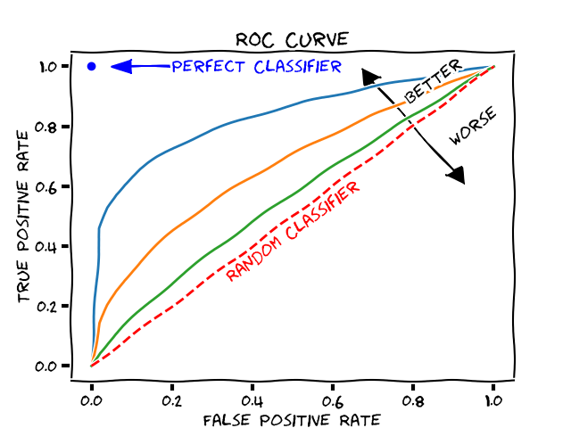
The ROC curve is a graphical plot that shows how a binary classifier changes when a threshold value is changed.

Final Notes

Think about the smoke detector case. We don't have a positive example here, so we can't estimate the classifiers quality on it. Please note that there is literature about estimating the probability of a rare event - even if you have never observed it. But estimating the probability in general is something different then classifying it - for the classification part you need to know some characteristics of the event.