Maximum Fixed-Length Contiguous Subarray

I recently taught a course about improving code for performance. An obvious performance improvement is to not execute unnecessary operations. I lacked a good example when I gave the course, but here is one: Find value of the largest contiguous sub-array of fixed length in a huge array.

This is a toy example, of course, but it shows the idea quite well.

The Code is on GitHub.

Small Example

Input:

• array: [7, 9, 2, 0, 5, 2, 0, 1, 1, 2]
• sub-array length m = 3

Contiguous sub-arrays of the given length:

1. [7, 9, 2], value = 18
2. [9, 2, 0], value = 11
3. [2, 0, 5], value = 7
4. [0, 5, 2], value = 7
5. [5, 2, 0], value = 7
6. [2, 0, 1], value = 3
7. [0, 1, 1], value = 2
8. [1, 1, 2], value = 4

Output: 18

Inefficient Solution

The following solution makes use of the slicing notation. It is short, easy to read and mostly pretty efficient:

from typing import List


def find_biggest_subarray_slice(array: List[int], m: int) -> int:
    return max(sum(array[i : i + m]) for i in range(len(array) - m + 1))

Except that it has one flaw: It makes too many additions and accesses list elements way more often than necessary

Efficient Solution

from typing import List


def find_biggest_subarray_iterative(array: List[int], m: int) -> int:
    value = sum(array[0:m])
    largest_sub_array = value
    for remove, add in zip(array, array[m:]):
        value = value - remove + add
        largest_sub_array = max(value, largest_sub_array)
    return largest_sub_array

Comparison

The inefficient solution is in $\mathcal{O}((n - m) \cdot m)$, the efficient one is in $\mathcal{O}(n - m)$. So you will notice the difference clearly when you compare the execution times with big $m$.

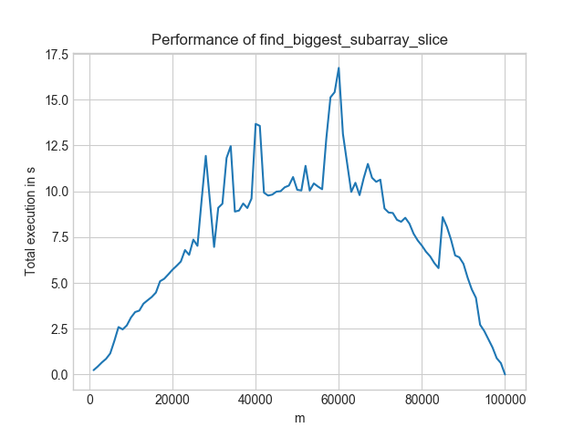
The inefficient solution changes its execution time like as shown in the image below for increasing m and contant n = 100,000:

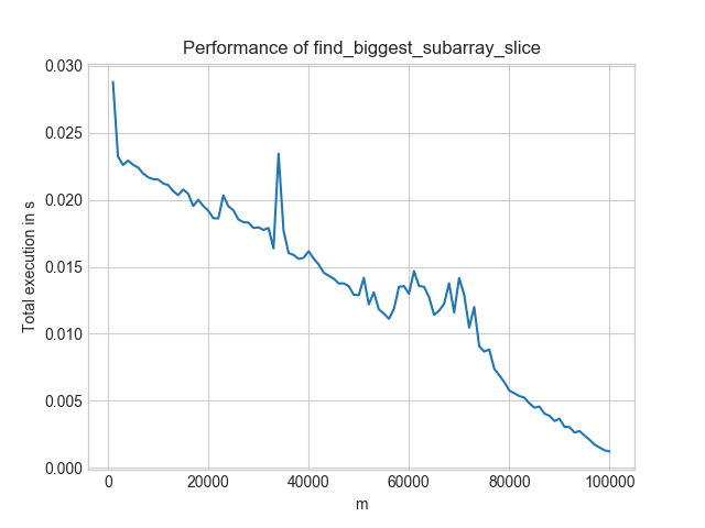
In contrast, the efficient solution looks like this:

Two things to notice:

• Worst-Case: For the inefficient solution, it is $m = n/2$. For the efficient solution, it is $m = 1$.
• Level: The efficient solution is always below 0.03s. The inefficient one is only for the best-case scenario ($n=m$) below that. And even then, the efficient solution is at 0.0008s whereas the inefficient one is at 0.001s.
• Speed-ups: If you look at $m = 60,000$, the more efficient solution gives a 1000× speedup!

See also

• Maximum Contiguous Subarray Sum