I was recently quite disappointed by how bad neural networks are for function approximation (see How should a neural network for unbound function approximation be structured?). However, I've just found that Gaussian processes are great for function approximation!
There are two important types of function approximation:
- Interpolation: What values does the function have in between of known values?
- Extrapolation: What values does the function have outsive of the known values?
I did a couple of very quick examples which look promising.
Examples
Square
Approximating $f(x) = x^2$ worked very good:
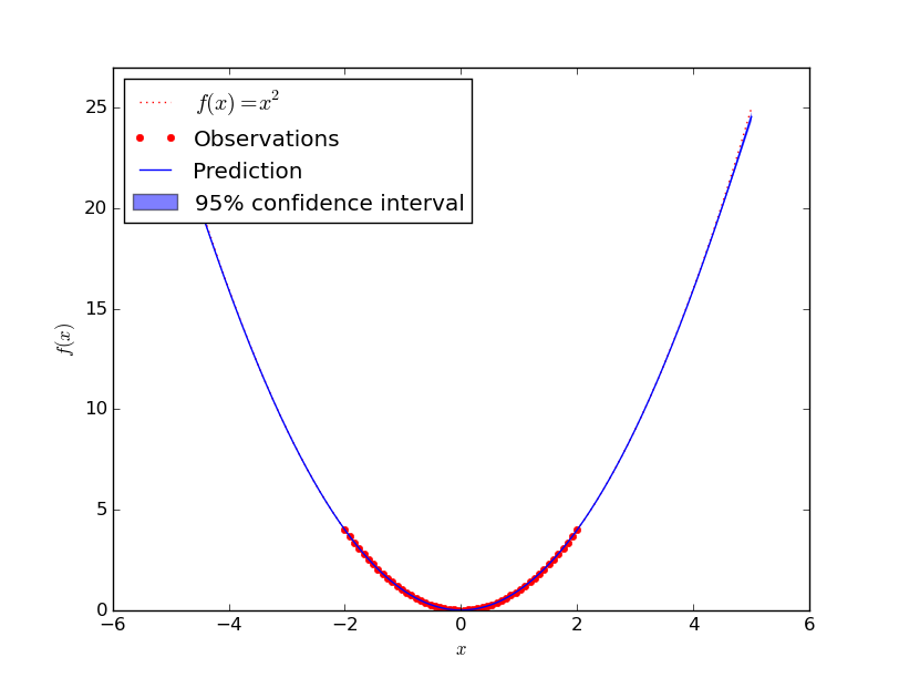
I've tried if with higher order polynomials, more complex polynomials. No problem.
Sin
Approximating $f(x) = \sin(3x)$ seems to be more complicated:
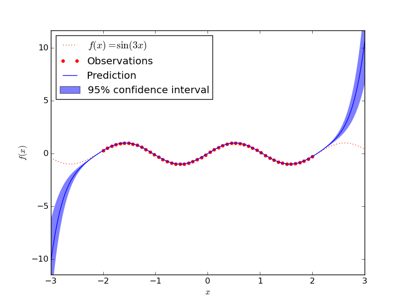
I guess a human would see the wave pattern and do a better job here.
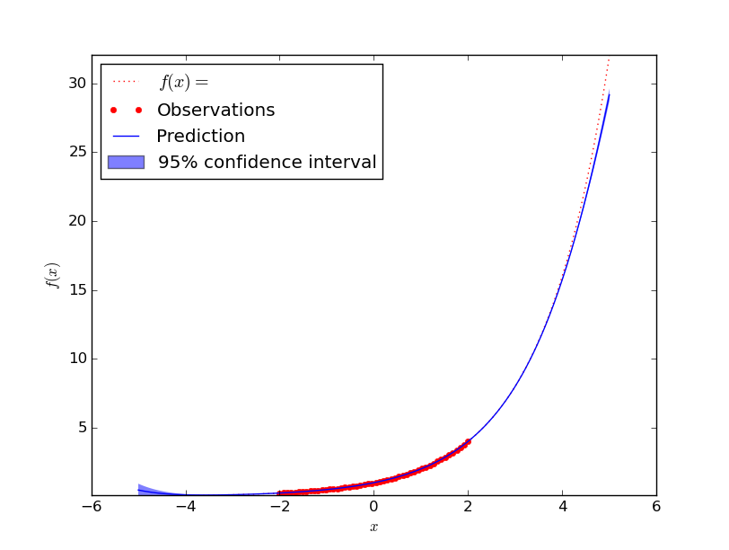
exp
Approximating $f(x) = e^x$ works similar well as polynomials. One can see that it does not perfectly fit it, but compared the the range of values seen before and the distance from the last seen value I think this is absolutely acceptable:
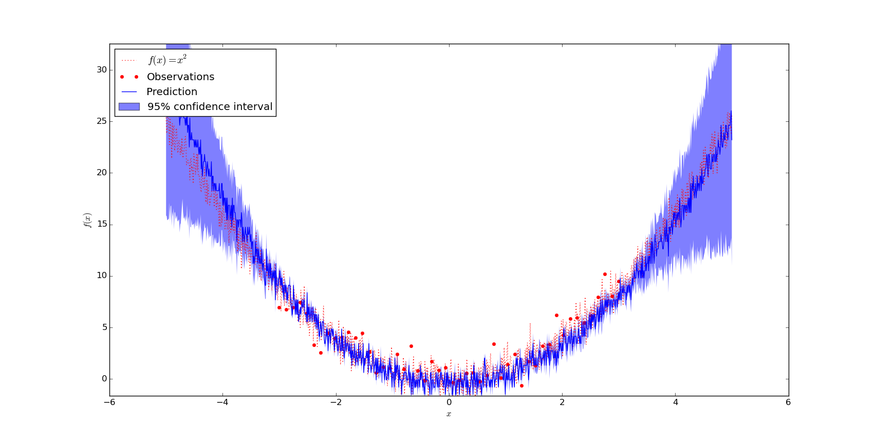
noise
It is claimed that Gaussian processes implicitly model noise so that they can easily deal with noise. However, in my experients this seems not to work so great. The reason might be that I had points in $[-3, 3]$ of the function
$$f(x) = x^2$$
with point-wise gaussian noise $N \sim \mathcal{N}(0, 1)$. So the noise is quite domintant on that intervall. One of the examples where it worked better is:
Make it brake
I was a bit suspicious if I had another mistake here. So I wanted it to break. This was the reason why I created the following function
$$f(x) = \begin{cases}x^2 &\text{if } x \geq 0\\-1 &\text{otherwise}\end{cases}$$
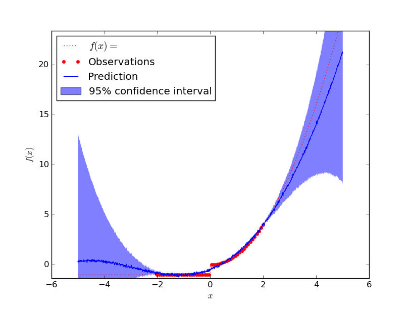
The predicted value is obviously not correct, but you should note that almost all function values are within the 95% confidence intervall!
Code
The following code needs numpy
and sklearn. For the plots,
you need matplotlib.
#!/usr/bin/env python

"""Example how to use gaussion processes for regression."""

import numpy as np
from sklearn import gaussian_process


def main():
    # Create the dataset
    x_train = np.atleast_2d(np.linspace(-3, 3, num=50)).T
    y_train = f(x_train).ravel()
    x_test = np.atleast_2d(np.linspace(-5, 5, 1000)).T

    # Define the Regression Modell and fit it
    gp = gaussian_process.GaussianProcess(theta0=1e-2, thetaL=1e-4, thetaU=1e-3)
    gp.fit(x_train, y_train)

    # Evaluate the result
    y_pred, mse = gp.predict(x_test, eval_MSE=True)
    print("MSE: %0.4f" % sum(mse))
    print("max MSE: %0.4f" % max(mse))
    plot_graph(x_test, x_train, y_pred, mse, "x^2")


def f(x):
    """
    Function which gets approximated
    """

    noise = [np.random.normal(loc=0.0, scale=1.0) for _ in range(len(list(x)))]
    noise = np.atleast_2d(noise).T
    return x ** 2 + noise
    # Totally fails for that one:
    # y = []
    # for el in x:
    #     if el >= 0:
    #         y.append(el**2)
    #     else:
    #         y.append(-1)
    # return np.array(y)


def plot_graph(x, x_train, y_pred, mse, function_tex):
    # Plot the function, the prediction and the 95% confidence interval
    # based on the MSE
    sigma = np.sqrt(mse)
    from matplotlib import pyplot as pl

    pl.figure()
    y = f(x_train).ravel()
    pl.plot(x, f(x), "r:", label="$f(x) = %s$" % function_tex)
    pl.plot(x_train, y, "r.", markersize=10, label="Observations")
    pl.plot(x, y_pred, "b-", label="Prediction")
    pl.fill(
        np.concatenate([x, x[::-1]]),
        np.concatenate([y_pred - 1.9600 * sigma, (y_pred + 1.9600 * sigma)[::-1]]),
        alpha=0.5,
        fc="b",
        ec="None",
        label="95% confidence interval",
    )
    pl.xlabel("$x$")
    pl.ylabel("$f(x)$")
    y_min = min(min(y_pred), min(y)) * 1.1
    y_max = max(max(y_pred), max(y)) * 1.1
    pl.ylim(y_min, y_max)
    pl.legend(loc="upper left")
    pl.show()


if __name__ == "__main__":
    main()
See also
- www.gaussianprocess.org: The definitive book about gaussian processes. It's freely available online!
- Wikipedia
- sklearn: Gaussian Processes
- sklearn: Gaussian Processes regression: basic introductory example