I am currently improving many articles on Wikipedia as a preparation for some math exams. And I recently started to create images with LaTeX / TikZ.
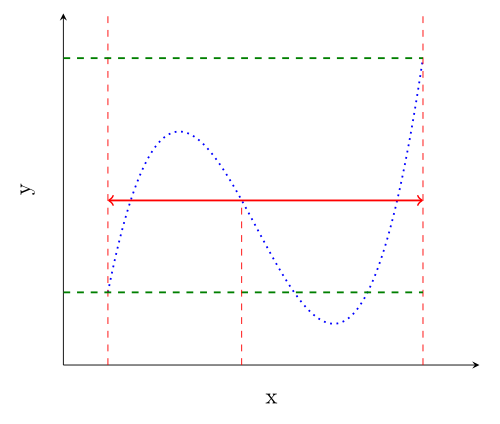
Today, I've found this image in the article about the Intermediate value theorem:
Get special points
As a first step, you should open the image with GIMP (or any other editor of your choice) and find the pixel-coordinates of special points:
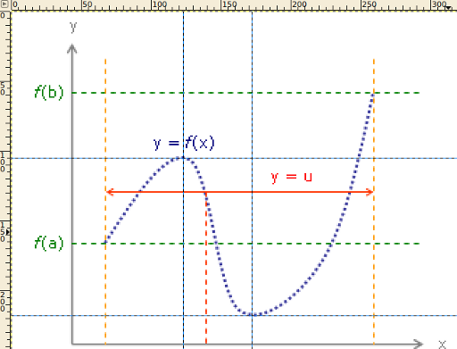
This function has a maximum at (123 | 105) and a minimum at (172 | 218) ... well, thats not correct. Note that the axis of GIMP starts at the upper left. So the y-axis is wrong.
I have cropped and flipped the image vertically. Now you can read the minimum / maximum coordinates with GIMP:
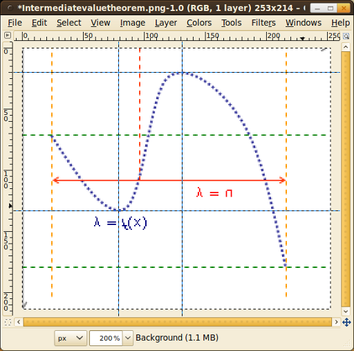
The local maximum is at (79 | 133) and the local minimum is at (131 | 20).
Form equations
A cubic function generally looks like this: $f(x) = a \cdot x^3 + b \cdot x^2 + c \cdot x + d$
You have two points, so they have to fit to this equation: (I) $f(79) = 133$ (II) $f(131) = 20$
The derivative has to be zero in a minimum and a maximum, so you know two more equations: (III) $f'(79) = 0$ (IV) $f'(131) = 0$
Four linear equations and four variables. Now we can solve those equations.
Get explicit equations
As a first step, we write down the equations in an explicit form. You have to know the general derivate of a cubic function: $f'(x) = 3 a\cdot x^2 + 2 b \cdot x + c$
(I) $493039a + 6241b+79c + d = 133$ (II) $2352637a + 17689b + 131c + d = 20$ (III) $18723a + 158 b + c = 0$ (IV) $51483 a + 262 b + c = 0$
Solve the equations
Now you have to solve the equations. I took Wolfram|Alpha, because the numbers are really ugly. If you like to do it by hand, you have to know how to use the Gaussian algorithm.
Here is the exact solution:

And here is an approximation:

The LaTeX Code
\documentclass{article}
\usepackage[pdftex,active,tightpage]{preview}
\setlength\PreviewBorder{2mm}
\usepackage{pgfplots}
\usepackage{units}
\pgfplotsset{compat=1.3}% <-- moves axis labels near ticklabels
                        % (respects tick label widths)
\usepackage{tikz}
\usetikzlibrary{arrows, positioning, calc, intersections, decorations.markings}

\usepackage{xcolor}
\definecolor{horizontalLineColor}{HTML}{008000}
\definecolor{verticalLineColor}{HTML}{FF0000}

\begin{document}

% Define this as a command to ensure that it is same in both cases
\newcommand*{\ShowIntersection}[2]{
\fill
    [name intersections={of=#1 and #2, name=i, total=\t}]
    [red, opacity=1, every node/.style={above left, black, opacity=1}]
    \foreach \s in {1,...,\t}{(i-\s) circle (2pt)
        node [above left] {\s}};
}

\begin{preview}
\begin{tikzpicture}
    \begin{axis}[
        label distance=0mm,
        width=8cm, height=7cm,     % size of the image
        xmin= 40,      % start the diagram at this x-coordinate
        xmax= 180,    % end   the diagram at this x-coordinate
        ymin=60,     % start the diagram at this y-coordinate
        ymax=170,   % end   the diagram at this y-coordinate
        ylabel=y,
        xlabel=x,
        axis lines=left,
        tick style={draw=none},
        xticklabels={,,},
        yticklabels={,,}
    ]
      \addplot[name path global=a, domain=55:161, dotted, blue,
               thick,samples=500, label=$y=f(x)$]
        {113/132078*x*x*x-11865/44026*x*x+1169437/44026*x-93155207/132078};
      % ( 55 |  82.7344) and (161 | 156.011) are on the graph
      \coordinate (b) at (axis cs: 55,170);
      \coordinate (c) at (axis cs:161,170);
      \coordinate (d) at (axis cs:161,82.7344);
      \coordinate (e) at (axis cs:161,156.011);
      \coordinate (a1) at (axis cs:55,111.494);
      \coordinate (a2) at (axis cs:161,111.494);
      \draw[verticalLineColor, thick, <->](a1) -- (a2);
      \draw[verticalLineColor,dashed](b |- 0,0) -- (b);
      \draw[verticalLineColor,dashed](c |- 0,0) -- (c);
      \draw[horizontalLineColor,dashed, thick](d -| 0,0) -- (d);
      \draw[horizontalLineColor,dashed, thick](e -| 0,0) -- (e);

      % (100 | 111.494)
      \coordinate (f) at (axis cs:100, 111.494);
      \draw[red,dashed](f |- 0,0) -- (f);
    \end{axis}
\end{tikzpicture}
\end{preview}
\end{document}
The result