Wie bildet man den Schnitt zweier Vektorräume?

· by

Inhalt
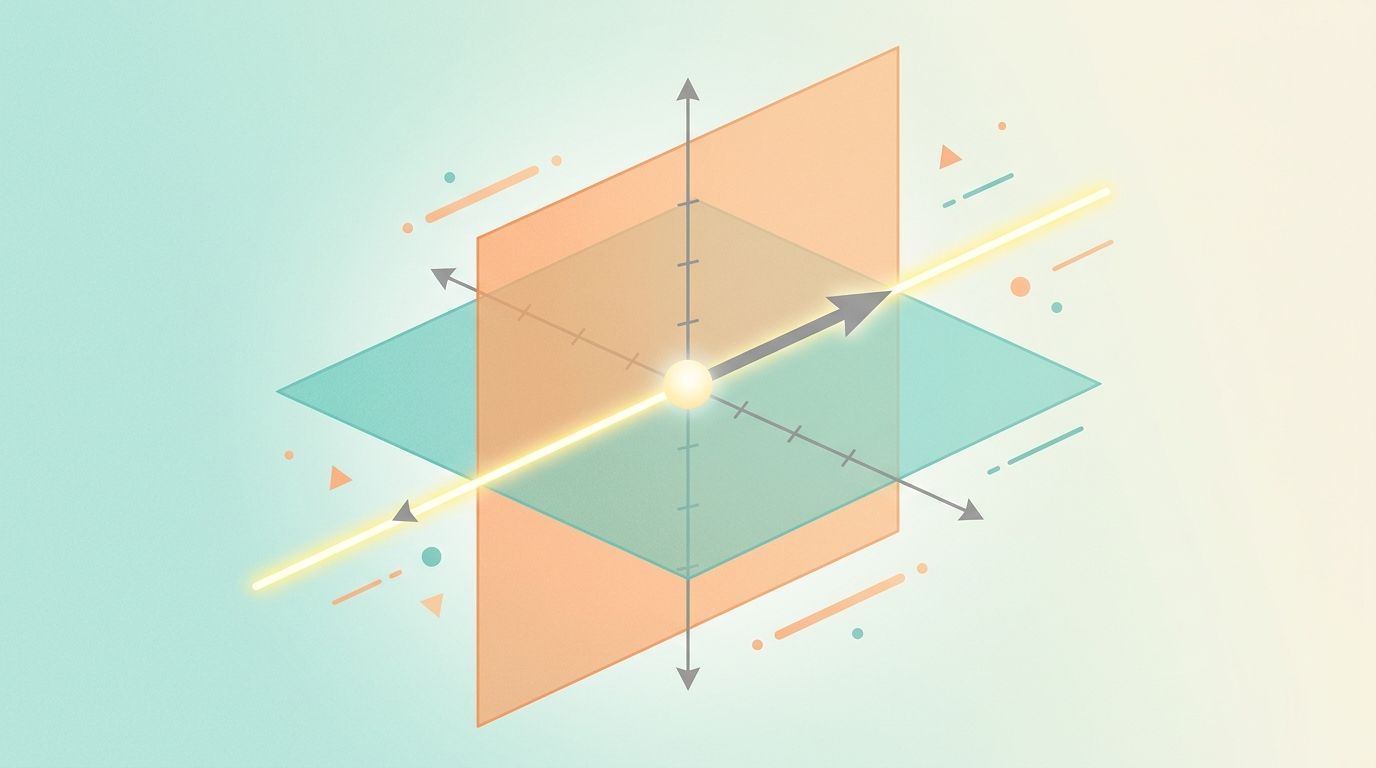
Zwei farbige Ebenen im Raum, die sich in einer Geraden schneiden, auf der ein Basisvektor eingezeichnet ist
Der Schnitt zweier Untervektorräume ist wieder ein Untervektorraum.

Angaben

Gegeben sind zwei Untervektorräume des \(\mathbb{R}^4\):

$$U_1 := \left [\begin{pmatrix} 2 \\ 5 \\ 3 \\ 17 \end{pmatrix}, \begin{pmatrix} 1 \\ 2 \\ 3 \\ 4 \end{pmatrix}, \begin{pmatrix} 1 \\ 3 \\ 3 \\ 7 \end{pmatrix}, \begin{pmatrix} -1 \\ 1 \\ -1 \\ 1 \end{pmatrix} \right ]$$
$$U_2 := \left [\begin{pmatrix} 0 \\ 0 \\ 4 \\ 2 \end{pmatrix}, \begin{pmatrix} 3 \\ 1 \\ 4 \\ 1 \end{pmatrix}, \begin{pmatrix} 2 \\ 7 \\ 1 \\ 8 \end{pmatrix}, \begin{pmatrix} 36 \\ 126 \\ 8 \\ 139 \end{pmatrix} \right ]$$

Aufgabe

Finde eine Basis für \(U_1 \cap U_2\).

Zusatzaufgabe: Finde eine Basis für \(U_1 + U_2\).

Basis finden

Will man eine möglichst einfache Basis, also ein minimales Erzeugendensystem mit möglichst kleinen Zahlen zu einem gegebenem Vektorraum finden, so kann man das Gaußsche Eliminationsverfahren auf die erzeugenden Vektoren anwenden. Dazu transponiert man die Vektoren:

$$\left( \begin{array}{c c c c | c} 2 & 5 & 3 & 17 & 0\\ 1 & 2 & 3 & 4 & 0\\ 1 & 3 & 3 & 7 & 0\\ -1 & 1 &-1 & 1 & 0 \end{array} \right)$$

Da im Gaußsche Eliminationsverfahren nur das Vertauschen von Zeilen, die Multiplikation einer Zeile mit einer Konstanten und die Addition von Zeilen zugelassen sind, bleibt die rechte Spalte immer Null. Sie kann also weggelassen werden:

$$\left( \begin{array}{c c c c} 2 & 5 & 3 & 17\\ 1 & 2 & 3 & 4\\ 1 & 3 & 3 & 7\\ -1 & 1 &-1 & 1 \end{array} \right) \rightsquigarrow \left( \begin{array}{c c c c} 1 &-1 & 1 &-1\\ 0 & 3 & 2 & 5\\ 0 & 4 & 2 & 8\\ 0 & 7 & 1 & 19 \end{array} \right) \rightsquigarrow \left( \begin{array}{c c c c} 1 &-1 & 1 &-1\\ 0 & 1 & \frac{1}{2} & 2\\ 0 & 0 & \frac{1}{2} & -1\\ 0 & 0 & -\frac{5}{2} & 5 \end{array} \right) \rightsquigarrow $$
$$\left( \begin{array}{c c c c} 1 &-1 & 1 &-1\\ 0 & 1 & \frac{1}{2} & 2\\ 0 & 0 & 1 & -2\\ 0 & 0 & -5 & 10 \end{array} \right) \rightsquigarrow \left( \begin{array}{c c c c} 1 & 0 & 0 & 4\\ 0 & 1 & 0 & 3\\ 0 & 0 & 1 & -2\\ 0 & 0 & 0 & 0 \end{array} \right)$$

Die Basis für \(U_1\) ist also

$$\left \{\begin{pmatrix} 1 \\ 0 \\ 0 \\ 4 \end{pmatrix}, \begin{pmatrix} 0 \\ 1 \\ 0 \\ 3 \end{pmatrix}, \begin{pmatrix} 0 \\ 0 \\ 1 \\ -2 \end{pmatrix} \right \}$$

Ich habe gerade keine Lust, das ganze für \(U_2\) noch vorzurechnen. Es kommt

$$\left( \begin{array}{c c c c} 1 & 0 & 0 & -\frac{29}{38}\\ 0 & 1 & 0 & \frac{49}{38}\\ 0 & 0 & 1 & \frac{1}{2}\\ 0 & 0 & 0 & 0 \end{array} \right)$$

heraus, siehe Wolfram|Alpha.

Die Basis für \(U_2\) ist also

$$\left \{\begin{pmatrix} 1 \\ 0 \\ 0 \\ -\frac{29}{38} \end{pmatrix}, \begin{pmatrix} 0 \\ 1 \\ 0 \\ \frac{49}{38} \end{pmatrix}, \begin{pmatrix} 0 \\ 0 \\ 1 \\ \frac{1}{2} \end{pmatrix} \right \}$$

Zassenhaus-Algorithmus

Man transponiert die Basisvektoren von \(U_1\) und \(U_2\) und schreibt sie in eine Matrix:

$$\left( \begin{array}{c | c} U_1^T & U_1^T \\ \hline U_2^T & 0 \end{array} \right)$$

Natürlich nimmt man für \(U_1\) und \(U_2\) die einfacheren Basen von oben. Dann löst man das ganze wieder mit Gauß. Im ersten Schritt zieht man von jeder der drei unteren Zeilen die entsprechende obere Zeile ab:

$$\left( \begin{array}{c c c c | c c c c} 1 & 0 & 0 & 4 & 1 & 0 & 0 & 4 \\ 0 & 1 & 0 & 3 & 0 & 1 & 0 & 3 \\ 0 & 0 & 1 &-2 & 0 & 0 & 1 &-2 \\ \hline 1 & 0 & 0 & - \frac{29}{38} & 0 & 0 & 0 & 0 \\ 0 & 1 & 0 & \frac{49}{38} & 0 & 0 & 0 & 0 \\ 0 & 0 & 1 & \frac{1}{2} & 0 & 0 & 0 & 0 \end{array} \right) \rightsquigarrow \left( \begin{array}{c c c c | c c c c} 1 & 0 & 0 & 4 & 1 & 0 & 0 & 4 \\ 0 & 1 & 0 & 3 & 0 & 1 & 0 & 3 \\ 0 & 0 & 1 &-2 & 0 & 0 & 1 &-2 \\ \hline 0 & 0 & 0 & - \frac{181}{38} & -1 & 0 & 0 & -4 \\ 0 & 0 & 0 & - \frac{65}{38} & 0 & -1 & 0 & -3 \\ 0 & 0 & 0 & \frac{5}{2} & 0 & 0 & -1 & 2 \end{array} \right) \rightsquigarrow $$

Die letzte Zeile wird mit \(\frac{2}{5}\) multipliziert und nach oben geschoben. Mit ihr eliminiert man die vierte Spalte in den beiden anderen unteren Zeilen:

$$\left( \begin{array}{c c c c | c c c c} 1 & 0 & 0 & 4 & 1 & 0 & 0 & 4 \\ 0 & 1 & 0 & 3 & 0 & 1 & 0 & 3 \\ 0 & 0 & 1 &-2 & 0 & 0 & 1 &-2 \\ 0 & 0 & 0 & 1 & 0 & 0 & - \frac{2}{5} & \frac{4}{5} \\ \hline 0 & 0 & 0 & 0 & -1 & 0 & - \frac{181}{95} & - \frac{18}{95} \\ 0 & 0 & 0 & 0 & 0 & -1 & - \frac{13}{19} & - \frac{31}{19} \end{array} \right) \rightsquigarrow \left( \begin{array}{c c c c | c c c c} 1 & 0 & 0 & 4 & 1 & 0 & 0 & 4 \\ 0 & 1 & 0 & 3 & 0 & 1 & 0 & 3 \\ 0 & 0 & 1 &-2 & 0 & 0 & 1 &-2 \\ 0 & 0 & 0 & 1 & 0 & 0 & - \frac{2}{5} & \frac{4}{5} \\ \hline 0 & 0 & 0 & 0 & 95 & 0 & 181 & 18 \\ 0 & 0 & 0 & 0 & 0 & 19 & 13 & 31 \end{array} \right)$$

(Im letzten Schritt wurden die beiden unteren Zeilen mit \(-95\) bzw. \(-19\) multipliziert.)

Rechts unten steht nun die Basis für \(U_1 \cap U_2 = \left [ \left \{ \begin{pmatrix} 95 \\ 0 \\ 181 \\ 18 \end{pmatrix}, \begin{pmatrix} 0 \\ 19 \\ 13 \\ 31 \end{pmatrix} \right \} \right ]\). Zusätzlich steht links oben die Basis für \(U_1 + U_2\). Wenn man das noch etwas umformt ist es die Standardbasis des \(\mathbb{R}^4\).

Zur Probe: Beide Vektoren liegen in \(U_1\), denn für jeden Vektor aus \(U_1\) gilt \(x_4 = 4 x_1 + 3 x_2 - 2 x_3\) (also \(380 - 362 = 18\) und \(57 - 26 = 31\)). Sie liegen auch in \(U_2\), denn dort gilt \(x_4 = -\frac{29}{38} x_1 + \frac{49}{38} x_2 + \frac{1}{2} x_3\) (also \(-\frac{145}{2} + \frac{181}{2} = 18\) und \(\frac{49}{2} + \frac{13}{2} = 31\)). Auch die Dimensionen passen: \(\dim(U_1 \cap U_2) = \dim U_1 + \dim U_2 - \dim(U_1 + U_2) = 3 + 3 - 4 = 2\).

Methode 2

Angabe

$$U_1 = \left [ \left \{\begin{pmatrix} 1 \\ 0 \\ 0 \\ 4 \end{pmatrix}, \begin{pmatrix} 0 \\ 1 \\ 0 \\ 3 \end{pmatrix}, \begin{pmatrix} 0 \\ 0 \\ 1 \\ -2 \end{pmatrix} \right \} \right ]$$
$$U_2 = \left [ \left \{\begin{pmatrix} 1 \\ 0 \\ 0 \\ -\frac{29}{38} \end{pmatrix}, \begin{pmatrix} 0 \\ 1 \\ 0 \\ \frac{49}{38} \end{pmatrix}, \begin{pmatrix} 0 \\ 0 \\ 1 \\ \frac{1}{2} \end{pmatrix} \right \} \right ]$$

Rechnung

Es gilt: \(x \in U_1 \cap U_2\) \(\Leftrightarrow x \in U_1 \land x \in U_2\) \(\Leftrightarrow x = a \cdot x_1 + b \cdot x_2 + c \cdot x_3 = -(d \cdot y_1 + e \cdot y_2 + f \cdot y_3)\) mit \(a, b, c, d, e, f \in \mathbb{R}\), also \(a \cdot x_1 + b \cdot x_2 + c \cdot x_3 + d \cdot y_1 + e \cdot y_2 + f \cdot y_3 = 0\).

$$\begin{pmatrix} 1 & 0 & 0 & 1 & 0 & 0\\ 0 & 1 & 0 & 0 & 1 & 0\\ 0 & 0 & 1 & 0 & 0 & 1\\ 4 & 3 & -2 & -\frac{29}{38} & \frac{49}{38} & \frac{1}{2} \end{pmatrix} \rightsquigarrow \begin{pmatrix} 1 & 0 & 0 & 1 & 0 & 0\\ 0 & 1 & 0 & 0 & 1 & 0\\ 0 & 0 & 1 & 0 & 0 & 1\\ 0 & 0 & 0 & -\frac{181}{38} & -\frac{65}{38} & \frac{5}{2} \end{pmatrix}$$
$$\rightsquigarrow \begin{pmatrix} 1 & 0 & 0 & 1 & 0 & 0\\ 0 & 1 & 0 & 0 & 1 & 0\\ 0 & 0 & 1 & 0 & 0 & 1\\ 0 & 0 & 0 & 1 & \frac{65}{181} & -\frac{95}{181} \end{pmatrix} \rightsquigarrow \begin{pmatrix} 1 & 0 & 0 & 0 & -\frac{65}{181} & \frac{95}{181}\\ 0 & 1 & 0 & 0 & 1 & 0\\ 0 & 0 & 1 & 0 & 0 & 1\\ 0 & 0 & 0 & 1 & \frac{65}{181} & -\frac{95}{181} \end{pmatrix}$$

Nun führt der \(-1\) - Trick zu dieser Lösung:

$$\mathcal{L} = \left [ \left \{ \begin{pmatrix} -\frac{65}{181} \\ 1 \\ 0 \\ \frac{65}{181} \\ -1 \\ 0\end{pmatrix}, \begin{pmatrix} \frac{95}{181} \\ 0 \\ 1 \\ -\frac{95}{181} \\ 0 \\ -1 \end{pmatrix} \right \} \right ] = \left [ \left \{ \begin{pmatrix} -65 \\ 181 \\ 0 \\ 65 \\ -181 \\ 0\end{pmatrix}, \begin{pmatrix} 95 \\ 0 \\ 181 \\ -95 \\ 0 \\ -181 \end{pmatrix} \right \} \right ]$$

Das ist also die Lösung für Belegungen von a, b, c, d, e, f, sodass der resultierende Vektor sowohl in \(U_1\), als auch in \(U_2\) ist. Setzt man \(a, b, c\) in \(x = a \cdot x_1 + b \cdot x_2 + c \cdot x_3\) ein, erhält man

$$U_1 \cap U_2 = \left [ \left \{ \begin{pmatrix} -65 \\ 181 \\ 0 \\ 283 \end{pmatrix}, \begin{pmatrix} 95 \\ 0 \\ 181 \\ 18 \end{pmatrix} \right \} \right ]$$

Das ist derselbe Raum wie beim Zassenhaus-Algorithmus, nur mit einer anderen Basis: Der zweite Vektor kommt dort direkt vor, und \(\begin{pmatrix} -65 \\ 181 \\ 0 \\ 283 \end{pmatrix} = -\frac{13}{19} \begin{pmatrix} 95 \\ 0 \\ 181 \\ 18 \end{pmatrix} + \frac{181}{19} \begin{pmatrix} 0 \\ 19 \\ 13 \\ 31 \end{pmatrix}\).
Siehe auch

Interaktiver Zassenhaus-Algorithmus